Sorting#
We will now explore several algorithms aimed at solving the sorting problem:
Input: A sequence of \(n\) numbers \(< a_1, a_2, \ldots, a_n >\)
Output: A permutation (reordering) \(< a_1', a_2', \ldots, a_n' >\) of the input sequence such that \(a_1' \leq a_2' \leq \cdots \leq a_n'\)
Set Interface#
Storing items in an array in arbitrary order can implement a set (though not the most efficient approach). Sorting the stored items by key allows:
Quick retrieval of min and max values (at the first and last index of the array).
Rapid search using binary search, achieving \(O(\log n)\) time complexity.
Data Structure |
Container |
Static |
Dynamic |
Dynamic |
Dynamic |
|---|---|---|---|---|---|
insert(x) |
find_min() |
find_prev(i) |
|||
build(x) |
find(k) |
delete(k) |
find_max() |
find_next(k) |
|
Array |
\(n\) |
\(n\) |
\(n\) |
\(n\) |
\(n\) |
Sorted Array |
\(n \log n\) |
\(\log n\) |
\(n\) |
\(1\) |
\(\log n\) |
Operations comparison of different data structures - \(O(\cdot)\). This table was removed from the lecture 3 notes of the class Introduction to Algorithms [DKS20].
In-Place Algorithm#
An in-place algorithm is one that operates directly on its input data without requiring extra space proportional to the input size. In other words, it doesn’t use additional memory to perform its task. Instead, it typically rearranges elements of the input data structure, such as an array or a list, in a way that avoids needing additional storage.
\(\textcolor{#FFC0D9}{\Longrightarrow}\) Memory Efficiency: In-place algorithms are memory efficient as they modify the input data structure without using additional space.
\(\textcolor{#FFC0D9}{\Longrightarrow}\) Space Complexity: They typically have a space complexity of \(O(1)\), meaning constant extra space is used.
Non In-Place Algorithm#
A non in-place algorithm requires additional space proportional to the size of the input to perform its task. It may use extra memory for creating data structures or managing state during computation.
\(\textcolor{#FFC0D9}{\Longrightarrow}\) Additional Space: Non in-place algorithms may use \(O(n)\) or more space, where \(n\) is the size of the input.
\(\textcolor{#FFC0D9}{\Longrightarrow}\) Flexibility: They can be more flexible in approach and may achieve better time complexity by utilizing extra memory.
Permutation Sort#
\(\textcolor{#FFC0D9}{\Longrightarrow}\) Permutation Sort - Time complexity : \(\Omega(n! \cdot n\))
The pseudocode for permutation sort is shown in Algorithm \ref{algo:perm_sort}. There are \(n!\) permutations of the set \(A\), and at least one of these permutations will be sorted. For each permutation, we check whether it is sorted in \(\Theta(n)\) time. Regarding the analysis, we can confirm its correctness by case analysis, as it tries all possibilities (brute force). Since the implementation of the function permutations(A) is unknown, we must assume \(\Omega(\cdot)\) instead of \(O(\cdot)\). Consequently, verifying if a permutation is sorted takes \(O(n)\), and going through all possible permutations takes \(\Omega(n!)\). Therefore, the total time complexity is \(\Omega(n! \cdot n)\).
def permutation_sort(A):
    """
    Perform permutation sort on array A.
    Time complexity: Ω(n! * n)
    """
    from itertools import permutations

    for B in permutations(A):  # Ω(n!)
        if list(B) == sorted(A):  # O(n)
            return list(B)  # O(1)

A = [-1, -10, -5, 1, 5, 7, 0, -2, 10, -5, -2]
print(f"Unsorted array: {A}")
permutation_sort(A)
print(f"Sorted array: {A}")
Unsorted array: [-1, -10, -5, 1, 5, 7, 0, -2, 10, -5, -2]
Sorted array: [-1, -10, -5, 1, 5, 7, 0, -2, 10, -5, -2]
Insertion Sort#
\(\textcolor{#FFC0D9}{\Longrightarrow}\) Insertion Sort (in-place) - Time complexity : \(\Theta(n^2)\) | Space complexity : \(O(1)\)
Insertion Sort is a simple and intuitive sorting algorithm that builds the final sorted array (or list) one item at a time. It is much like the way you might sort playing cards in your hands. Based on the algorithm \ref{algo:insert_sort} let’s analyze the loop invariant and the correctness of insertion sort. Loop Invariant:
Initialization: it’s true prior to the first iteration of the loop
Maintenance: it’s true before an iteration of the loop, it remains true before the next iteration
Termination: when the loop terminates, the invariant gives us a useful property that helps show that the algorithm is correct
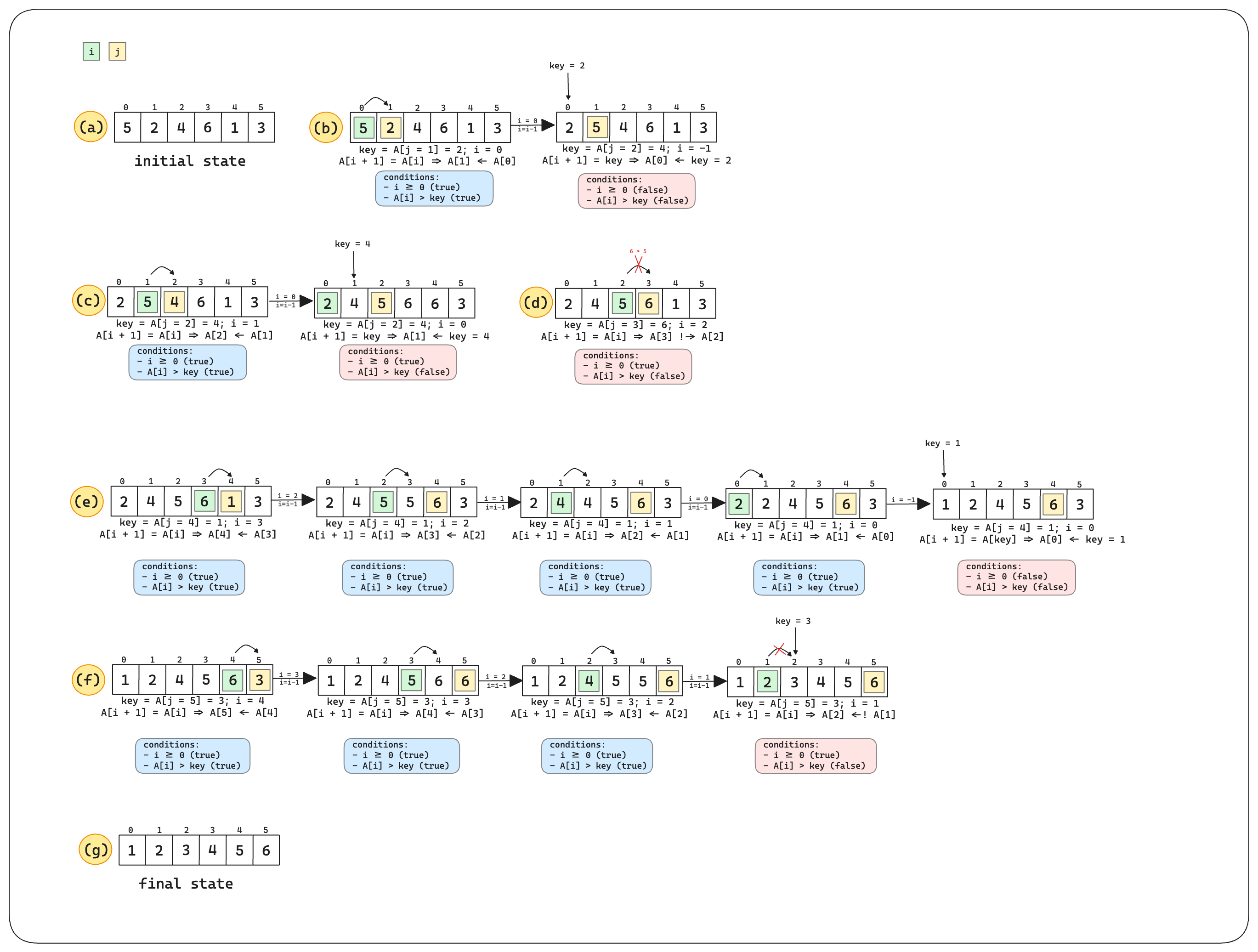
Fig. 3 Insertion sort illustration.#
def insertion_sort(A):
    """
    Perform insertion sort on array A.
    Time complexity: Θ(n^2)
    """
    for j in range(1, len(A)):  # Θ(n)
        key = A[j]  # insert A[j] into the sorted sequence A[1, ..., j-1]
        i = j - 1
        while i >= 0 and A[i] > key:  # Θ(n)
            A[i + 1] = A[i]
            i = i - 1
        A[i + 1] = key
    return A


A = [-1, -10, -5, 1, 5, 7, 0, -2, 10, -5, -2]
print(f"Unsorted array: {A}")
insertion_sort(A)
print(f"Sorted array: {A}")
Unsorted array: [-1, -10, -5, 1, 5, 7, 0, -2, 10, -5, -2]
Sorted array: [-10, -5, -5, -2, -2, -1, 0, 1, 5, 7, 10]
Merge Sort#
\(\textcolor{#FFC0D9}{\Longrightarrow}\) Merge Sort (Non in-place) - Time complexity : \(\Theta(n \log n)\) | Space complexity : \(O(n)\)
Merge Sort is an efficient, stable, and comparison-based sorting algorithm that follows the divide-and-conquer paradigm. It divides the input array into two halves, sorts each half, and then merges the two sorted halves. The code for this algorithm was divided into two parts: merge and merge-sort. A schematic of the algorithm can be seen in the figure below. In general we have:
Divide the problem into smaller subproblems
Conquer the subproblems by solving them recursively
Combine the solutions into one final answer
For the merge method, each basic step of comparing two elements at a time takes constant time. However, we perform at most n comparisons thus merging takes \(\Theta(n)\).
Running time of the divide-and-conquer part#
We can solve this problem using the substitution method. Let’s start with the hypothesis that \(T(n) = O(n \log n)\). For Merge Sort, the recurrence relation is \(T(n) = 2T(\lfloor n/2 \rfloor) + cn\). Assuming that the number of elements is a power of two, we have:
Using the strategy of finding a negative value, we need to find a \(\delta\) such that:
This results in:
We need
to show that \(\delta > 0\). Assuming \(\log 2 = 1\), we have:
\(\textcolor{#FFC0D9}{\Longrightarrow}\) Hence, by mathematical induction, if \(T(n) \leq d n \log(n) - d n \log(2) + cn\) is true, and \(d n \log(n) \geq d n \log(n) - d n \log(2) + cn\), then \(T(n) \leq d n \log(n)\). Therefore, \(\Theta(n \log(n))\).
def merge(A, p, q, r):
    """
    Merge subarrays of A.
    Time complexity: Θ(n)
    """
    n1 = q - p + 1
    n2 = r - q
    L = A[p:q + 1] + [float('inf')]
    R = A[q + 1:r + 1] + [float('inf')]
    i = j = 0

    for k in range(p, r + 1):
        if L[i] <= R[j]:
            A[k] = L[i]
            i += 1
        else:
            A[k] = R[j]
            j += 1

def merge_sort(A, p, r):
    """
    Perform merge sort on array A.
    Time complexity: Θ(n log n)
    """
    if p < r:
        q = (p + r) // 2
        merge_sort(A, p, q)
        merge_sort(A, q + 1, r)
        merge(A, p, q, r)
    return A

A = [-1, -10, -5, 1, 5, 7, 0, -2, 10, -5, -2]
print(f"Unsorted array: {A}")
merge_sort(A, 0, len(A) - 1)
print(f"Sorted array: {A}")
Unsorted array: [-1, -10, -5, 1, 5, 7, 0, -2, 10, -5, -2]
Sorted array: [-10, -5, -5, -2, -2, -1, 0, 1, 5, 7, 10]

Fig. 4 Merge Sort Schematic.#
Bubble Sort#
\(\textcolor{#FFC0D9}{\Longrightarrow}\) Bubble Sort (in-place) - Time complexity: \(\Theta(n^2)\) | Space complexity: \(O(1)\)
def bubble_sort(A):
    """
    Perform bubble sort on array A.
    Time complexity: Θ(n^2)
    """
    n = len(A)
    for i in range(n - 1):
        for j in range(n - i - 1):
            if A[j] > A[j + 1]:
                A[j], A[j + 1] = A[j + 1], A[j]

A = [-1, -10, -5, 1, 5, 7, 0, -2, 10, -5, -2]
print(f"Unsorted array: {A}")
bubble_sort(A)
print(f"Sorted array: {A}")
Unsorted array: [-1, -10, -5, 1, 5, 7, 0, -2, 10, -5, -2]
Sorted array: [-10, -5, -5, -2, -2, -1, 0, 1, 5, 7, 10]
Time Complexity#
We start at the beginning of the array and move downward, possibly swapping elements, until we reach the previously sorted subsection of the array. Each iteration increases in steps or performs fewer comparisons. The total number of comparisons can be approximated by summing up the iterations:
This simplifies to \(\Theta(n^2)\). This quadratic time complexity arises because in the worst case, we may need to compare each element with every other element, resulting in a total time proportional to \( n^2 \).
\(\textcolor{#FFC0D9}{\Longrightarrow}\) Note that the best case scenario for insertion sort is \(\Theta(n)\) whereas for bubble sort is \(\Theta(n^2)\)
Heap Sort#
\(\textcolor{#FFC0D9}{\Longrightarrow}\) Heap Sort (in-place) - Time complexity: \(O(n \log n)\) | Space complexity: \(O(1)\)
Heaps#
The binary heap is a data structure represented as an array that forms a nearly complete binary tree. It has some base operations as shown below and it adheres to specific heap properties:
max-heap: each parent node is greater than or equal to its children.
min-heap: each parent node is less than or equal to its children.
To visualize how we can conceive a binary tree given a list please refer to the schematic in figure Illustration on how to conceive a binary tree..
Viewing a heap as a tree, we define the height of a node in a heap to be the number of edges on the longest simple downward path from the node to a leaf and we define the height of the heap to be the height of its root.
def parent(i):
    return i // 2

def left(i):
    return 2 * i + 1

def right(i):
    return 2 * i + 2
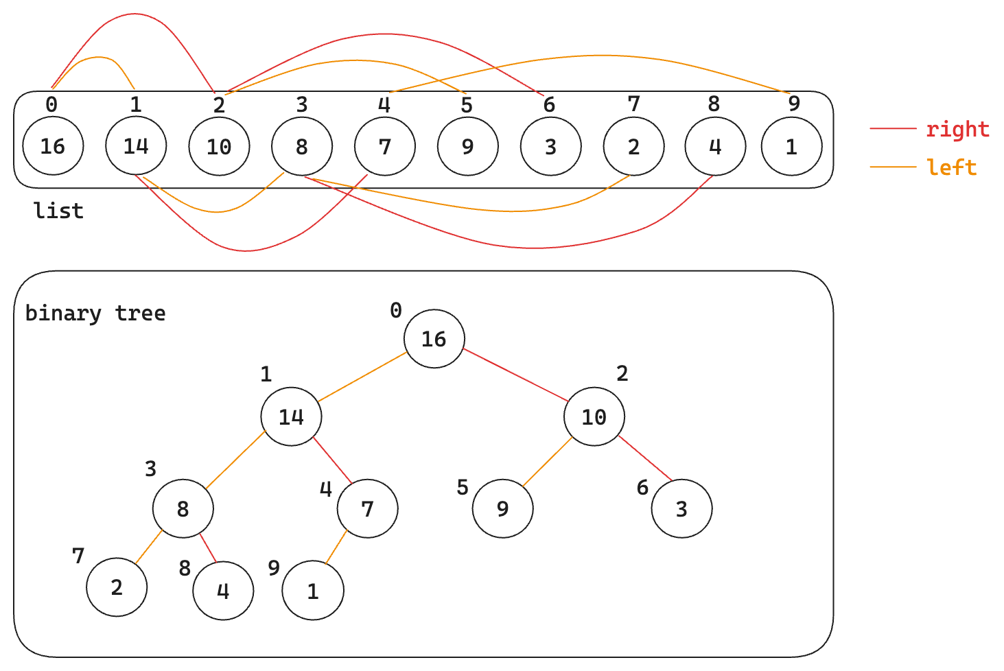
Fig. 5 Illustration on how to conceive a binary tree.#
Note
Since a heap of \(n\) elements is based on a complete binary tree, its height is \(\Theta(\log n)\).
Note
The basic operations of heaps run in a time at most proportional to the height of the tree and thus take \(O(\log n)\) time.
Maintaining the heap property#
In order to maintain the max-heap property, the procedure max_heapify is called.
def max_heapify(A, i, heap_size):
    """
    Maintain the max-heap property.
    """
    largest = i
    l = left(i)
    r = right(i)

    if l < heap_size and A[l] > A[largest]:
        largest = l
    if r < heap_size and A[r] > A[largest]:
        largest = r
    if largest != i:
        A[i], A[largest] = A[largest], A[i]
        max_heapify(A, largest, heap_size)

Fig. 6 Illustration of how max-heapify works.#
Building a Heap#
We can use the procedure max_heapify in a bottom-up manner to convert an array \(A[0 \ldots n]\) into a max-heap.
def build_max_heap(A):
    """
    Build a max-heap from array A.
    """
    heap_size = len(A)
    for i in range(len(A) // 2 - 1, -1, -1):
        max_heapify(A, i, heap_size)
We can compute a simple upper bound on the running time of build_max_heap as follows:
Each call to
max_heapifycosts \(O(\log n)\) time.build_max_heapmakes \(O(n)\) such calls.Thus, the running time is \(O(n \log n)\).
However, this upper bound, though correct, is not asymptotically tight.
Note
An \(n\)-element heap has height \(\lfloor \log n \rfloor\) and at most \(\lceil \frac{n}{2^{h+1}} \rceil\) nodes of any height \(h\).
Based on the information provided above, we can derive a tighter running time for build_max_heap, which is linear. Specifically, build_max_heap has a running time of \(O(n)\). For more details on these mathematical formulations, please refer to Chapter 6, Section 4 of the CLRS book [DKS20].
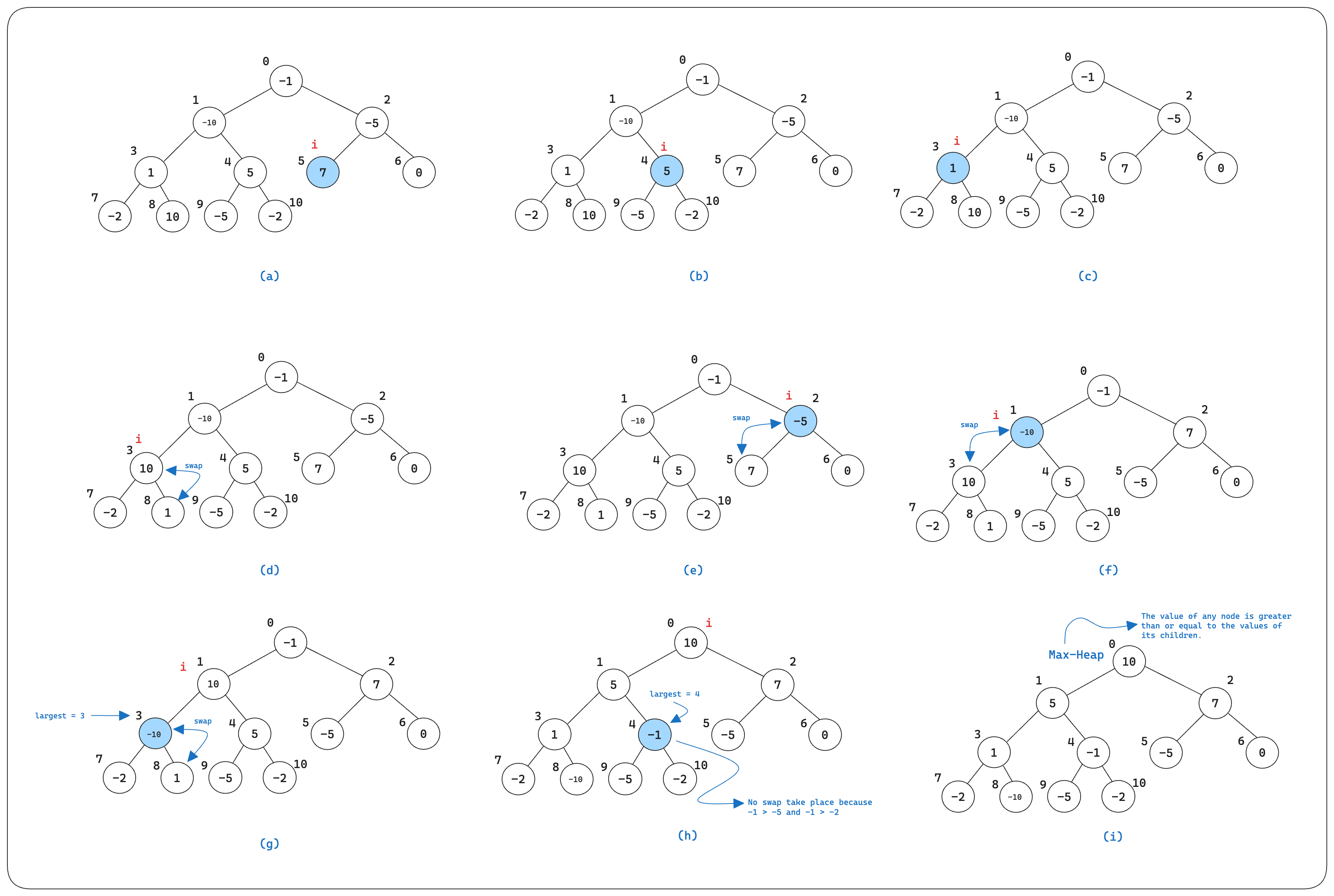
Fig. 7 Illustration of how build-max-heap works.#
Animation MaxHeap#
At Last, the Heapsort Algorithm#
The heapsort algorithm starts by using build_max_heap to build a max-heap on the input array \(A[ \ldots n]\), where \(n = A.length\).
def heap_sort(A):
    """
    Perform heapsort on array A.
    """
    build_max_heap(A)
    heap_size = len(A)
    for i in range(len(A) - 1, 0, -1):
        A[0], A[i] = A[i], A[0]
        heap_size -= 1
        max_heapify(A, 0, heap_size)
    return A

A = [-1, -10, -5, 1, 5, 7, 0, -2, 10, -5, -2]
print(f"Unsorted array: {A}")
heap_sort(A)
print(f"Sorted array: {A}")
Unsorted array: [-1, -10, -5, 1, 5, 7, 0, -2, 10, -5, -2]
Sorted array: [-10, -5, -5, -2, -2, -1, 0, 1, 5, 7, 10]
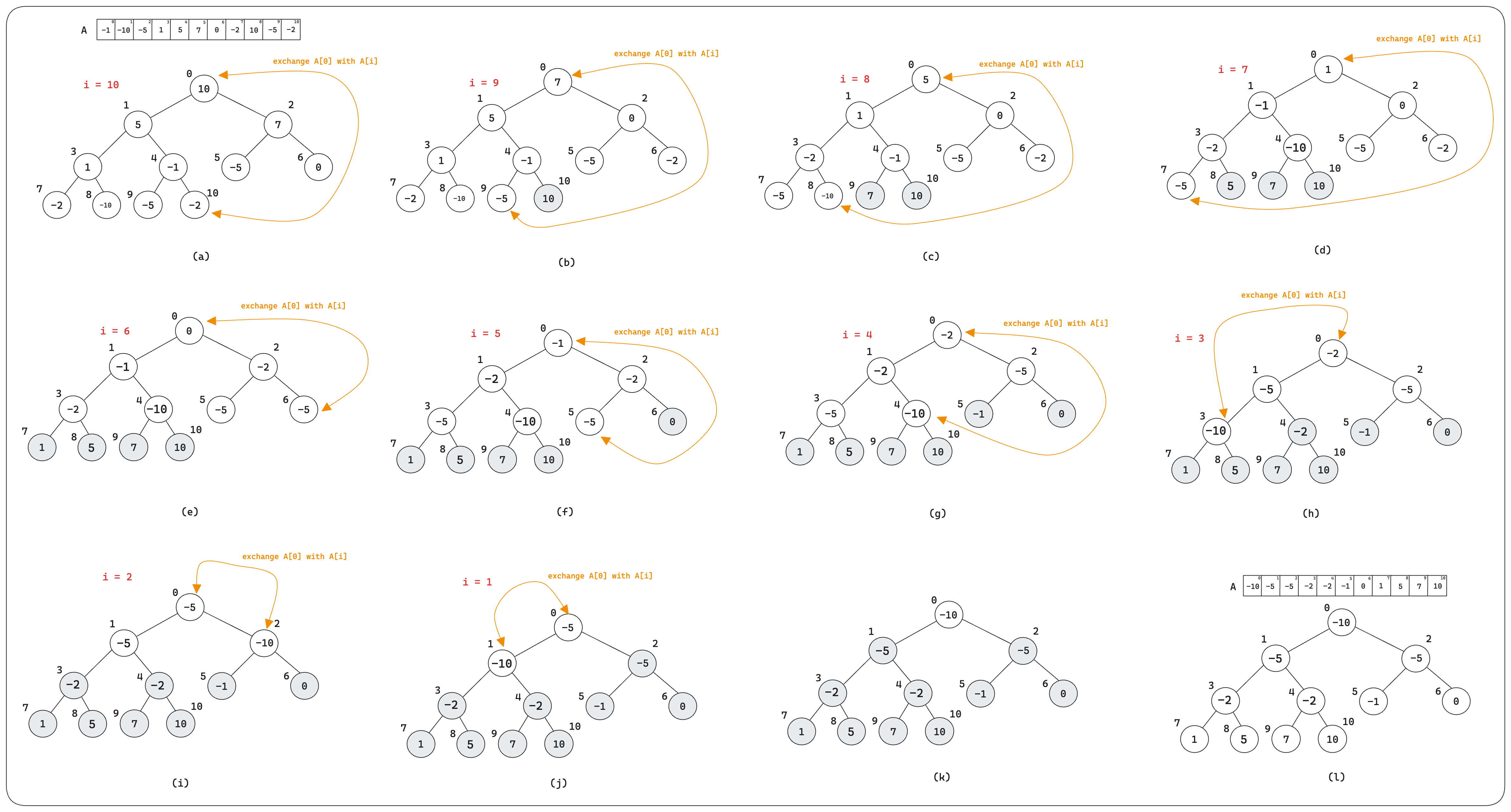
Fig. 8 Illustration of the heap sort process.#
Animation Heap Sort#
Quick Sort#
\(\textcolor{#FFC0D9}{\Longrightarrow}\) Quick Sort (in-place) - Time complexity: \(\Theta(n \log n)\) | Space complexity: \(O(1)\) | Worst case running time: \(\Theta(n^2)\)
Quick Sort is a highly efficient sorting algorithm that uses the divide-and-conquer strategy. The algorithm works as follows:
Choose a pivot element from the array.
Partition the array into two sub-arrays: elements less than the pivot and elements greater than the pivot.
Recursively apply the above steps to the sub-arrays.
Combine the sub-arrays to produce the sorted array.
def partition(A, p, r):
    """
    Partition the array A.
    Time complexity: Θ(n)
    """
    x = A[r]
    i = p - 1
    for j in range(p, r):
        if A[j] <= x:
            i += 1
            A[i], A[j] = A[j], A[i]
    A[i + 1], A[r] = A[r], A[i + 1]
    return i + 1

def quicksort(A, p, r):
    """
    Perform quicksort on array A.
    Time complexity: Θ(n log n)
    """
    if p < r:
        q = partition(A, p, r)
        quicksort(A, p, q - 1)
        quicksort(A, q + 1, r)
    return A

A = [-1, -10, -5, 1, 5, 7, 0, -2, 10, -5, -2]
print(f"Unsorted array: {A}")
sorted_A = quicksort(A, 0, len(A) - 1)
print(f"Sorted array: {sorted_A}")
Unsorted array: [-1, -10, -5, 1, 5, 7, 0, -2, 10, -5, -2]
Sorted array: [-10, -5, -5, -2, -2, -1, 0, 1, 5, 7, 10]
Performance of quicksort#
The running time of quicksort depends on whether the partitioning is balanced or unbalanced.
Note
If the partitioning is balanced, the algorithm runs asymptotically as fast as merge sort.
Note
If the partitioning is unbalanced, the algorithm runs asymptotically as slowly as insertion sort.
Worst-case partitioning#
The worst-case scenario for quicksort occurs when the partitioning process results in one subproblem with \(n - 1\) elements and another with \(0\) elements. For example, if the array is already sorted in ascending order and the pivot chosen is always the last element, quicksort will exhibit its worst-case behavior. Such a scenario yields a \(\Theta(n^2)\) running time.
Best-case partitioning#
In the best-case scenario, the partitioning process of quicksort divides the array into two nearly equal subarrays (one of size \(\lfloor n/2 \rfloor\) and one of size \(\lfloor n/2 \rfloor\)). This means that each pivot chosen perfectly splits the array such that the sizes of the subarrays are as balanced as possible, ideally with each containing roughly half of the elements. When this occurs, the depth of the recursion is minimized, and the overall time complexity of quicksort is reduced to \(\Theta(n \log n)\). That is,
[ T(n) = 2T(n/2) + \Theta(n) \implies T(n) = \Theta(n \log n) ]
This balanced partitioning ensures that the workload is evenly distributed across the recursive calls, resulting in efficient sorting performance.
Balanced partitioning#
The average-case running time of quicksort is significantly closer to the best-case scenario than to the worst-case scenario. This means that the performance of quicksort largely depends on the relative ordering of the elements in the input array rather than the specific values of the elements. For instance, if the elements are distributed in such a way that each pivot results in two subarrays of nearly equal size, quicksort will efficiently sort the array. An example of this is an array where the elements are randomly shuffled, leading to balanced partitions during the sorting process.
A randomized version of quicksort#
In examining the average-case behavior of quicksort, we assume that all permutations of the input array are equally likely. However, this assumption may not always hold in practice. To address this, we can use a randomized version of quicksort, which helps ensure that the pivot selection is not influenced by the initial ordering of the elements. By randomly selecting the pivot, we aim to achieve more balanced partitions on average, thereby improving the algorithm’s performance.
import random

def randomized_partition(A, p, r):
    """
    Randomized partitioning of the array A.
    """
    i = random.randint(p, r)
    A[r], A[i] = A[i], A[r]
    return partition(A, p, r)

def randomized_quicksort(A, p, r):
    """
    Perform randomized quicksort on array A.
    """
    if p < r:
        q = randomized_partition(A, p, r)
        randomized_quicksort(A, p, q - 1)
        randomized_quicksort(A, q + 1, r)
    return A

A = [-1, -10, -5, 1, 5, 7, 0, -2, 10, -5, -2]
print(f"Unsorted array: {A}")
sorted_A = randomized_quicksort(A, 0, len(A) - 1)
print(f"Sorted array: {sorted_A}")
Unsorted array: [-1, -10, -5, 1, 5, 7, 0, -2, 10, -5, -2]
Sorted array: [-10, -5, -5, -2, -2, -1, 0, 1, 5, 7, 10]
\(\textcolor{#FFC0D9}{\Longrightarrow}\) I recommend reading this Quora discussion, as it includes comments from one of the authors of the CLRS book, which we are using as a reference for this summary.
Thomas Cormen: “Both the deterministic and randomized quicksort algorithms have the same best-case running times of \(O(n\log(n))\) and the same worst-case running times of \(O(n^2)\). The difference is that with the deterministic algorithm, a particular input can elicit that worst-case behavior. With the randomized algorithm, however, no input can always elicit the worst-case behavior. The reason it matters is that, depending on how partitioning is implemented, an input that is already sorted–or almost sorted–can elicit the worst-case behavior in deterministic quicksort.”
Animation QuickSort#
Radix Sort#
\(\textcolor{#FFC0D9}{\Longrightarrow}\) Radix Sort - Time complexity: \(\Theta(d \cdot (n + k))\) | Space complexity: \(O(n + k)\)
Radix Sort is a non-comparative sorting algorithm that sorts numbers by processing individual digits. It operates by sorting the elements digit by digit, starting from the least significant digit (LSD) to the most significant digit (MSD). To achieve this, Radix Sort leverages a stable subroutine, such as Counting Sort, to sort the elements based on each digit. This ensures that the relative order of elements with equal digits is maintained, resulting in a stable sort.
The key idea behind Radix Sort is to treat the elements as strings of digits and process each digit position independently. This approach can be highly efficient for sorting large numbers of small integers or fixed-length strings.
def counting_sort(A, exp):
    """
    A function to do counting sort of A according to the digit represented by exp.
    """
    n = len(A)
    output = [0] * n
    count = [0] * 10

    for i in range(n):
        index = A[i] // exp
        count[index % 10] += 1

    for i in range(1, 10):
        count[i] += count[i - 1]

    i = n - 1
    while i >= 0:
        index = A[i] // exp
        output[count[index % 10] - 1] = A[i]
        count[index % 10] -= 1
        i -= 1

    for i in range(n):
        A[i] = output[i]

def radix_sort(A):
    """
    Perform radix sort on array A.
    """
    max1 = max(A)
    exp = 1
    while max1 // exp > 0:
        counting_sort(A, exp)
        exp *= 10

# Example usage
A = [170, 45, 75, 90, 802, 24, 2, 66]
print(f"Unsorted array: {A}")
radix_sort(A)
print(f"Sorted array: {A}")
Unsorted array: [170, 45, 75, 90, 802, 24, 2, 66]
Sorted array: [2, 24, 45, 66, 75, 90, 170, 802]
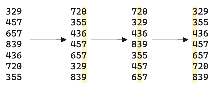
Fig. 9 Illustration of the radix sort process.#
Time Complexity Comparison#
Algorithm |
Time Complexity |
In-place? |
Stable? |
Comments |
|---|---|---|---|---|
Bubble Sort |
\(\Theta(n^2)\) |
Yes |
Yes |
Simple but inefficient for large datasets |
Selection Sort |
\(\Theta(n^2)\) |
Yes |
No |
Always performs \(\frac{n(n-1)}{2}\) comparisons |
Insertion Sort |
\(\Theta(n^2)\) |
Yes |
Yes |
Efficient for small or nearly sorted datasets |
Merge Sort |
\(\Theta(n \log n)\) |
No |
Yes |
Requires additional space for merging |
Quick Sort |
\(\Theta(n \log n)\) |
Yes |
No |
Fast but worst-case \(\Theta(n^2)\); randomization helps |
Heap Sort |
\(\Theta(n \log n)\) |
Yes |
No |
Good worst-case performance, not stable |
Counting Sort |
\(\Theta(n + u)\) |
No |
Yes |
\(O(n)\) when \(u = O(n)\) |
Radix Sort |
\(\Theta(d \cdot (n + k))\) |
No |
Yes |
Efficient for integers or fixed-length strings |
