Computing Time Complexity#
Computing the time complexity of algorithms can be challenging. Understanding and analyzing the time complexity is crucial for evaluating the efficiency of algorithms. Several methods are available to compute and solve recurrences, which help in determining the time complexity of recursive algorithms. In this section, we will briefly explain some commonly used methods and give some examples to sharpen our intuition.
Let’s focus on some examples and rules that can help determine the running time of an algorithm.
Examples:
Loops: The total running time is the product of the running time of the statements inside the loop and the number of iterations. In general, this results in \(O(n)\).
def simple_loop(n):
    for i in range(n):
        print("•")  # This statement runs n times
Nested Loops: The total running time is the product of the sizes of all the loops. For two nested loops, \(T(n) = c \cdot n \cdot n = cn^2 = O(n^2)\).
def nested_loops(n):
    for i in range(n):
        for j in range(n):
            print("•")  # This statement runs n * n times
Consecutive Statements: Add the time complexity of each statement. Look at the pseudocode in Algorithm, we have \(T(n) = c + cn + cn^2 = O(n^2)\).
def consecutive_statements_example(n):
    # Step 1
    print("•")  # Time Complexity: c
    # Step 2
    for i in range(n + 1):
        print("•")  # Time Complexity: cn
        # Step 3
        for j in range(n + 1):
            print("•")  # Time Complexity: cn^2
If-Then-Else: The total running time will be based on the test plus the larger of either part of the if/else. Look at Algorithm. We can see that \(T(n) = c + cn = O(n)\).
def if_then_else_example(n):
    # Step 1
    print("•")  # Time Complexity: c

    # Step 2
    if n == 1:
        print("•")  # Time Complexity: c
    else:
        # Step 3
        for i in range(n + 1):
            print("•")  # Time Complexity: cn
Tricky Example:
Sometimes, loops do not result in \(O(n)\) but rather \(O(\log n)\). Consider the example shown below. In this example, the for loop runs \(i\) times, but at each iteration, we multiply the value of \(i\) by 2. To understand the total running time, consider the following steps:
Iteration 1: \(i = 1 \rightarrow 2^0\)
Iteration 2: \(i = 2 \rightarrow 2^1\)
Iteration 3: \(i = 3 \rightarrow 2^2\)
Iteration 4: \(i = 4 \rightarrow 2^3\)
And so on, up to iteration k: \(i = n \rightarrow 2^{k-1}\)
Then, we can obtain a relation between \(k\) and \(n\).
Thus, we have \(O(\log n)\) as the time complexity since \(i\) is not growing linearly, but exponentially.
def tricky_for_loop(n):
    i = 1
    while i <= n:
        print("•")  # Comment: O(log i)
        i *= 2
Divide-and-Conquer#
Before diving into each method for solving the time complexity problem, let’s first understand a strategy called “divide-and-conquer,” which is very common in algorithms.
Divide-and-conquer is a technique where a problem is divided into smaller subproblems that are similar to the original problem but smaller in size. These subproblems are solved independently, and their solutions are combined to solve the original problem. This approach is particularly effective for problems that can be naturally divided into independent subproblems, leading to efficient recursive algorithms. Examples of divide-and-conquer algorithms include Merge Sort and Quick Sort, which use this technique to achieve optimal time complexities.
Recurrences#
A recurrence is an equation or inequality that describes a function in terms of its value on smaller inputs.
The maximum-subarray problem#
Our goal is to find the subarray which has the largest sum, with the constraint that the subarray must consist of adjacent elements from the original array.
A brute-force solution#
For this brute force solution let’s consider a window size of 2. An array of \(n\) items has \(\binom{n}{2}\) such pairs of subarrays. Since \(\binom{n}{2}\) is \(\Theta(n^2)\), and the best we can hope for is to evaluate each pair in constant time, this approach would take \(\Omega(n^2)\) time.
A solution using divide-and-conquer#
Let’s consider the scenario described in the CLRS book. The goal is to determine which subarray maximizes our profit given that we buy stocks when they are cheap and sell them when the price is higher than the purchase cost. We have an array representing the price fluctuations within a given time range and another array representing the price difference (change) every two consecutive days, as shown below
Day |
0 |
1 |
2 |
3 |
\(\cdots\) |
|---|---|---|---|---|---|
Price |
100 |
113 |
110 |
85 |
\(\cdots\) |
Change |
- |
13 |
-3 |
-25 |
\(\cdots\) |
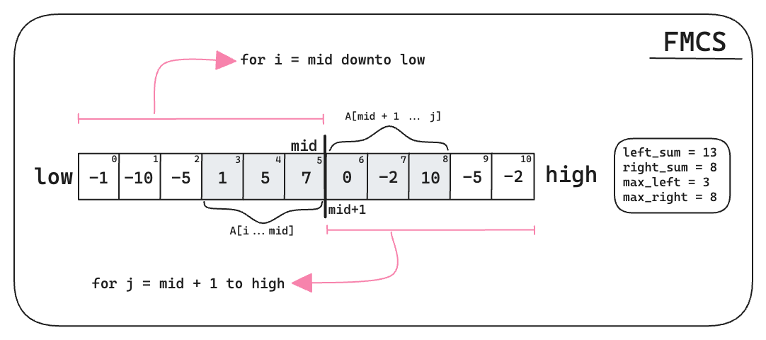
def find_maximum_crossing_subarray(A, low, mid, high):
    left_sum = float('-inf')
    _sum = 0
    max_left = mid

    for i in range(mid, low - 1, -1):
        _sum += A[i]
        if _sum > left_sum:
            left_sum = _sum
            max_left = i

    right_sum = float('-inf')
    _sum = 0
    max_right = mid + 1

    for j in range(mid + 1, high + 1):
        _sum += A[j]
        if _sum > right_sum:
            right_sum = _sum
            max_right = j

    return (max_left, max_right, left_sum + right_sum)

arr = [-1, -10, -5, 1, 5, 7, 0, -2, 10, -5, -2]
max_left, max_right, lr_sum = find_maximum_crossing_subarray(arr, 0, 5, 10)
print("max_left = ", max_left)
print("max_right = ", max_right)
print("left_sum + right_sum = ", lr_sum)
max_left =  3
max_right =  8
left_sum + right_sum =  21

Figure: Find Maximum Crossing Subarray Schematic
def find_maximum_subarray(A, low, high):
    # Base case
    if high == low:
        return (low, high, A[low])
    else:
        mid = (low + high) // 2
        left_low, left_high, left_sum = find_maximum_subarray(A, low, mid)
        right_low, right_high, right_sum = find_maximum_subarray(A, mid + 1, high)
        cross_low, cross_high, cross_sum = find_maximum_crossing_subarray(A, low, mid, high)

        if left_sum >= right_sum and left_sum >= cross_sum:
            return (left_low, left_high, left_sum)
        elif right_sum >= left_sum and right_sum >= cross_sum:
            return (right_low, right_high, right_sum)
        else:
            return (cross_low, cross_high, cross_sum)

# Example usage
arr = [-1, -10, -5, 1, 5, 7, 0, -2, 10, -5, -2]
low = 0
high = len(arr) - 1

result = find_maximum_subarray(arr, low, high)
print("Max left index:", result[0])
print("Max right index:", result[1])
print("Max sum:", result[2])
Max left index: 3
Max right index: 8
Max sum: 21

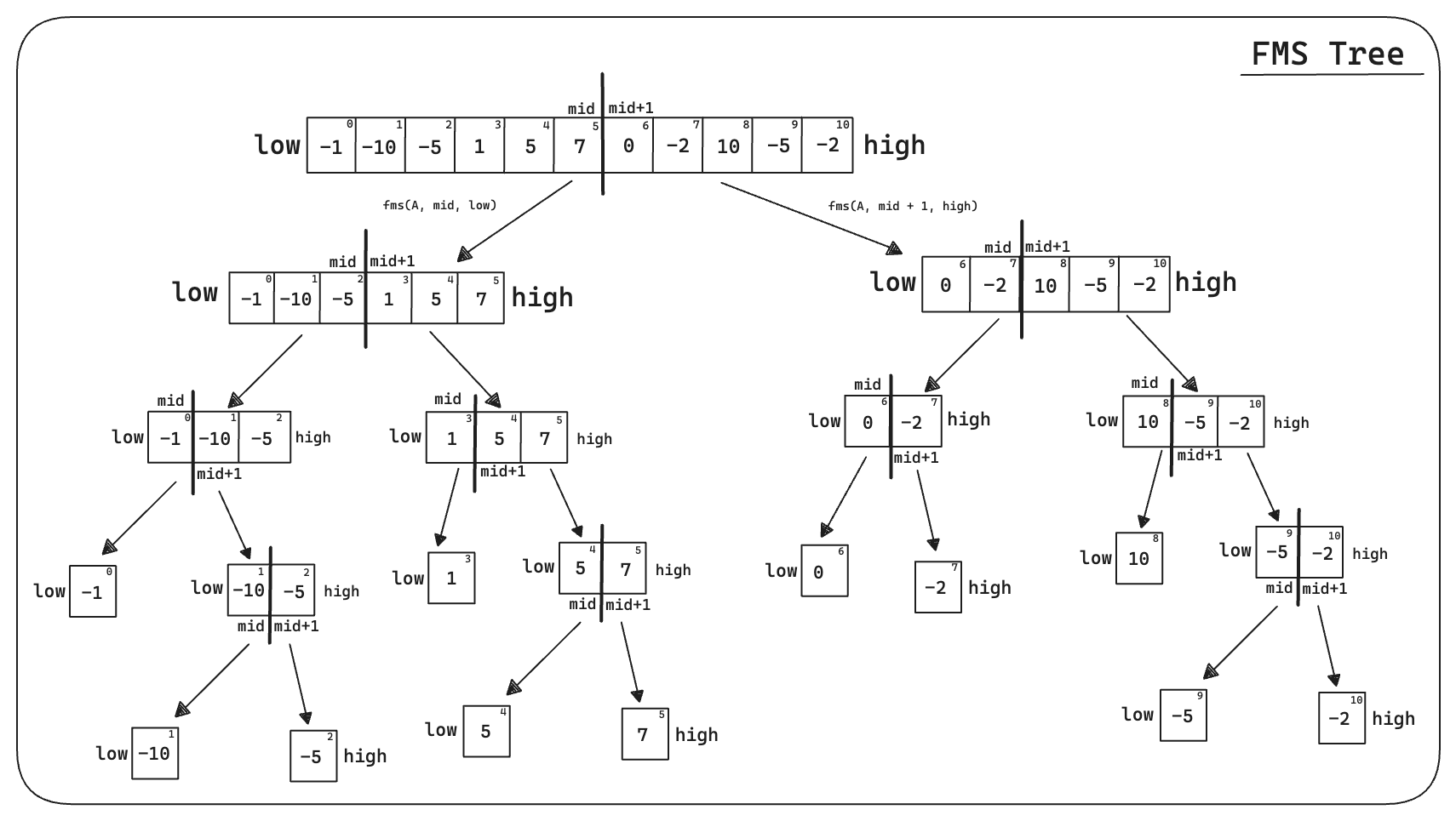
Figure:Find Maximum Subarray Tree Schematic
The codes shown above in find_maximum_subarray and find_maximum_crossing_subarray complement each other. The find_maximum_subarray function focuses on the divide and conquer strategy, splitting the problem into smaller parts and solving them. The find_maximum_crossing_subarray function, on the other hand, is responsible for calculating the maximum subarray that crosses the midpoint (mid). To analyze the algorithm’s complexity, we will use a method known as the recursion tree method. For a visualization on how the algorithm works please refer to the figures above. In addition, refer to the following animation with a step by step illustration:
Analyzing The Algorithm#
To perform our analysis, let’s assume that the original problem size is a power of 2. Denote \(T(n)\) as the running time for find_maximum_subarray on a subarray of \(n\) elements.
For the base case, when \(n = 1\), we have \(T(n) = \Theta(1)\) (constant time). The recursive case occurs when \(n > 1\). Each subproblem is solved on a subarray of \(n/2\) elements (our assumption that the original problem size is a power of 2 ensures that \(n/2\) is an integer), so we spend \(T(n/2)\) time solving each subproblem. Since we solve two subproblems, for the left and right subarrays, the time spent will be \(2T(n/2)\).
Next, we need to analyze the time for the find_maximum_crossing_subarray function. If the subarray \(A[\text{low} \cdots \text{high}]\) contains \(n\) entries (so that \(n = \text{high} - \text{low} + 1\)), we claim that find_maximum_crossing_subarray(A, low, mid, high) takes \(\Theta(n)\) time.
Since each iteration of the two for loops takes \(\Theta(1)\) time, we just need to count how many iterations there are altogether. The first for loop makes \(\text{mid} - \text{low} + 1\) iterations, and the second makes \(\text{high} - \text{mid}\) iterations. Thus, the total number of iterations is:
Hence, find_maximum_crossing_subarray takes linear time, \(\Theta(n)\).
Returning to our find_maximum_subarray method, the only remaining analysis concerns the if and else conditions, which all take constant time, \(\Theta(1)\). For the recursive case, we have:
Where fmcs is find_maximum_crossing_subarray and \([\cdot]\) is the comment from where this function is being considered either find_maximum_crossing_subarray or if-else. Thus,
We can express our running time \(T(n)\) for find_maximum_subarray as:
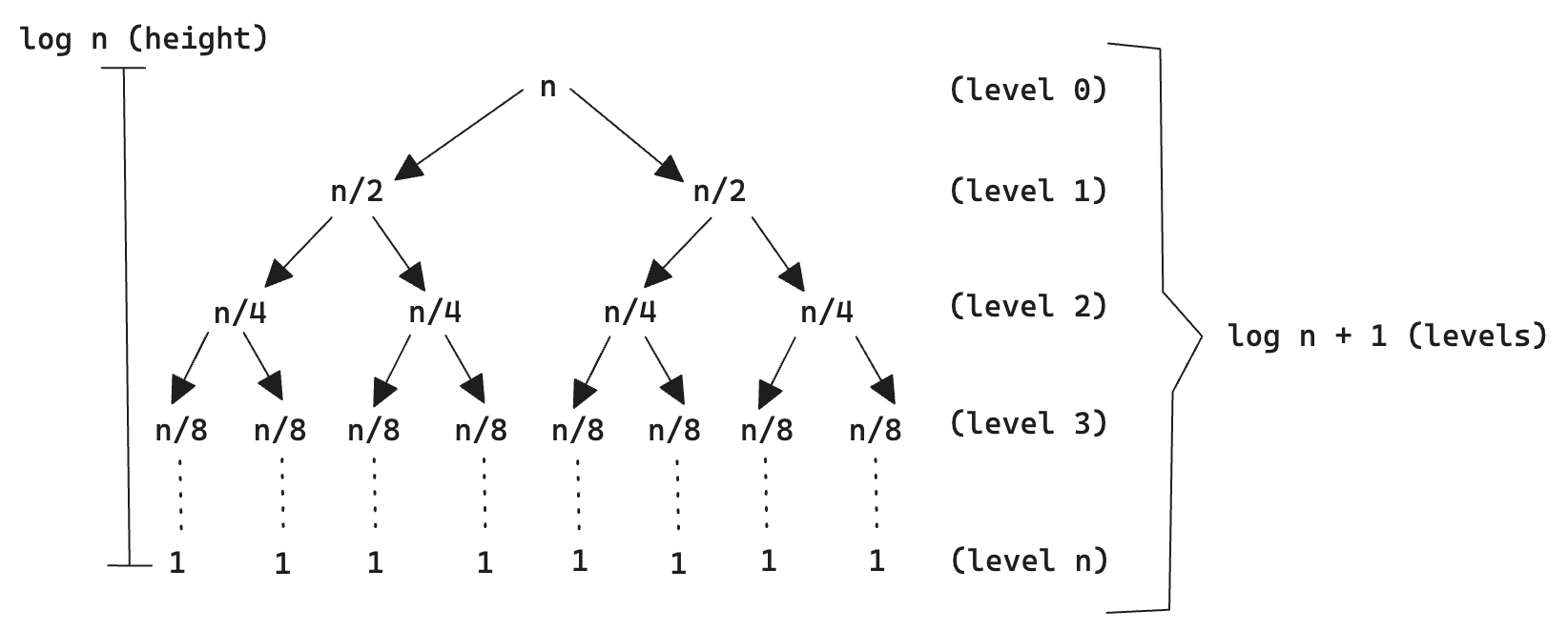
We will explore this in more detail in the next section, but a binary tree resulting from \(2T(n/2)\) has \(\log n + 1\) levels, and each level costs \(cn\) due to \(\Theta(n)\). Therefore,
Which then becomes,
Why the height of a binary tree is \(\log n\)?#
The height of the recursion tree is \(\log n\) because at each level of the recursion, the problem size is halved. That is, imagine our original problem size is a power of 2. Then
Initial Problem Size: Let’s start with a problem size of \(n\).
First Level: At the first level of recursion, the problem is divided into two subproblems, each of size \(n/2\).
Second Level: Each of these subproblems is further divided into two subproblems, each of size \(n/4\).
Subsequent Levels: This process continues, halving the problem size at each level.
Base Case: The recursion continues until the problem size is reduced to 1.
The number of levels in this recursion tree is the number of times we can divide \(n\) by 2 until we reach 1. This can be expressed as \(\log_2 n\). Formally, if we start with a problem of size \(n\) and divide it into halves, the height \(h\) of the recursion tree is given by:
So, the height of the tree is \(\log n\). The height of the tree is the level of the node(s) with the longest path to the root. To get a grasp of what is going on, please refer to the figure shown below:

Figure:Height and levels of a binary tree
\(\textcolor{#FFC0D9}{\Longrightarrow}\) The level of a node is its distance (each edge counts as 1) to the root node. So the root node has level 0, its direct children have level 1 etc - link. For binary trees, the number of levels is given by \(\log n + 1\).
\(\textcolor{#FFC0D9}{\Longrightarrow}\) The height of the tree is the level of the node(s) with the longest path to the root. Stated differently, the height is the maximum of all levels - link. For binary trees, the height is given by \(\log n\).
